Objective
An insurance company has been providing health insurance to its customers and are now hoping to build a model to predict whether the policy holders from past will also be interested in Vehicle Insurance provided by the company.
Building this model would help the company in its communication strategy to reach out to those customers and optimize its business model and revenue.
Now, in order to predict, whether the customer would be interested in Vehicle Insurance, the following information are at hand in the dataset,
- id
- Gender
- Age
- Driving_License - 0 : Customer does not have DL, 1 : Customer already has DL
- Region_Code
- Previously_Insured - 1 : Customer already has Vehicle Insurance, 0 : Customer doesn’t have Vehicle Insurance
- Vehicle_Age
- Vehicle_Damage - 1 : Customer got his/her vehicle damaged in the past. 0 : Customer didn’t get his/her vehicle damaged in the past
- Annual_Premium - The amount customer needs to pay as premium in the year
- PolicySalesChannel - Anonymized Code for the channel of outreaching to the customer ie. Different Agents, Over Mail, Over Phone, In Person, etc.
- Vintage - Number of Days, Customer has been associated with the company
- Response - 1 : Customer is interested, 0 : Customer is not interested
In this report, descriptive analytics and statistics is produced along with data preprocessing for the dataset. You can find the Github repo for this project here.
1. Load the data
1
2
3
4
5
6
7
8
9
| #the required libraries for the tasks are imported
import numpy as np #for efficient numerical operations
import pandas as pd #for manipulating and visualising data
import matplotlib.pyplot as plt #for data visualization
import seaborn as sns #for data visualization
#load the dataset
dataset = pd.read_csv('dataset.csv')
dataset.head(5)
|
| id | Gender | Age | Driving_License | Region_Code | Previously_Insured | Vehicle_Age | Vehicle_Damage | Annual_Premium | Policy_Sales_Channel | Vintage | Response |
|---|
| 0 | 1 | Male | 44 | 1 | 28 | 0 | > 2 Years | Yes | 40454 | 26 | 217 | 1 |
|---|
| 1 | 2 | Male | 76 | 1 | 3 | 0 | 1-2 Year | No | 33536 | 26 | 183 | 0 |
|---|
| 2 | 3 | Male | 47 | 1 | 28 | 0 | > 2 Years | Yes | 38294 | 26 | 27 | 1 |
|---|
| 3 | 4 | Male | 21 | 1 | 11 | 1 | < 1 Year | No | 28619 | 152 | 203 | 0 |
|---|
| 4 | 5 | Female | 29 | 1 | 41 | 1 | < 1 Year | No | 27496 | 152 | 39 | 0 |
|---|
2. Split the data into Training and Testing Dataset
1
2
3
4
5
6
7
| #import scikit-learn library for machine learning and also for sampling the dataset
from sklearn.model_selection import train_test_split
#the dataset is split into train and test dataset using random sampling
train, test = train_test_split(dataset, test_size=0.4, random_state = 7)
print(f"{train.shape[0]} train and {test.shape[0]} test instances")
|
228665 train and 152444 test instances
The dataset is split into train and test dataset. Train dataset alone would be used in this report to avoid data snooping.
1
2
| #to provide information on the train dataset
train.info()
|
1
2
3
4
5
6
7
8
9
10
11
12
13
14
15
16
17
18
19
| <class 'pandas.core.frame.DataFrame'>
Int64Index: 228665 entries, 301388 to 61615
Data columns (total 12 columns):
# Column Non-Null Count Dtype
--- ------ -------------- -----
0 id 228665 non-null int64
1 Gender 228665 non-null object
2 Age 228665 non-null int64
3 Driving_License 228665 non-null int64
4 Region_Code 228665 non-null int64
5 Previously_Insured 228665 non-null int64
6 Vehicle_Age 228665 non-null object
7 Vehicle_Damage 228665 non-null object
8 Annual_Premium 228665 non-null int64
9 Policy_Sales_Channel 228665 non-null int64
10 Vintage 228665 non-null int64
11 Response 228665 non-null int64
dtypes: int64(9), object(3)
memory usage: 22.7+ MB
|
1
2
| #to provide information on the test dataset
test.info()
|
1
2
3
4
5
6
7
8
9
10
11
12
13
14
15
16
17
18
19
| <class 'pandas.core.frame.DataFrame'>
Int64Index: 152444 entries, 87112 to 221223
Data columns (total 12 columns):
# Column Non-Null Count Dtype
--- ------ -------------- -----
0 id 152444 non-null int64
1 Gender 152444 non-null object
2 Age 152444 non-null int64
3 Driving_License 152444 non-null int64
4 Region_Code 152444 non-null int64
5 Previously_Insured 152444 non-null int64
6 Vehicle_Age 152444 non-null object
7 Vehicle_Damage 152444 non-null object
8 Annual_Premium 152444 non-null int64
9 Policy_Sales_Channel 152444 non-null int64
10 Vintage 152444 non-null int64
11 Response 152444 non-null int64
dtypes: int64(9), object(3)
memory usage: 15.1+ MB
|
Information on the train and test dataset can be seen above.
1
2
| #to check for null values
train.isnull().sum()
|
1
2
3
4
5
6
7
8
9
10
11
12
13
| id 0
Gender 0
Age 0
Driving_License 0
Region_Code 0
Previously_Insured 0
Vehicle_Age 0
Vehicle_Damage 0
Annual_Premium 0
Policy_Sales_Channel 0
Vintage 0
Response 0
dtype: int64
|
1
2
| #to check for null values
test.isnull().sum()
|
1
2
3
4
5
6
7
8
9
10
11
12
13
| id 0
Gender 0
Age 0
Driving_License 0
Region_Code 0
Previously_Insured 0
Vehicle_Age 0
Vehicle_Damage 0
Annual_Premium 0
Policy_Sales_Channel 0
Vintage 0
Response 0
dtype: int64
|
There are no missing values in the train and test dataset.
3. Exploratory Data Analysis
1
2
| #descriptive statistics on the train dataset
train.describe()
|
| id | Age | Driving_License | Region_Code | Previously_Insured | Annual_Premium | Policy_Sales_Channel | Vintage | Response |
|---|
| count | 228665.000000 | 228665.000000 | 228665.000000 | 228665.000000 | 228665.000000 | 228665.000000 | 228665.000000 | 228665.000000 | 228665.000000 |
|---|
| mean | 190652.209538 | 38.828557 | 0.997853 | 26.397398 | 0.458269 | 30595.860070 | 112.027350 | 154.434920 | 0.122940 |
|---|
| std | 110061.420927 | 15.535094 | 0.046289 | 13.222463 | 0.498257 | 17292.567811 | 54.194537 | 83.736668 | 0.328369 |
|---|
| min | 1.000000 | 20.000000 | 0.000000 | 0.000000 | 0.000000 | 2630.000000 | 1.000000 | 10.000000 | 0.000000 |
|---|
| 25% | 95377.000000 | 25.000000 | 1.000000 | 15.000000 | 0.000000 | 24432.000000 | 29.000000 | 82.000000 | 0.000000 |
|---|
| 50% | 190495.000000 | 36.000000 | 1.000000 | 28.000000 | 0.000000 | 31692.000000 | 131.000000 | 154.000000 | 0.000000 |
|---|
| 75% | 286007.000000 | 49.000000 | 1.000000 | 35.000000 | 1.000000 | 39432.000000 | 152.000000 | 227.000000 | 0.000000 |
|---|
| max | 381107.000000 | 85.000000 | 1.000000 | 52.000000 | 1.000000 | 540165.000000 | 163.000000 | 299.000000 | 1.000000 |
|---|
Descriptive statistics on the train dataset is seen above.
1
2
3
4
| #plot correlation matrix
plt.figure(figsize=(16,6))
ht=sns.heatmap(train.corr(), vmin=-1, vmax=1, annot=True)
ht.set_title('Correlation Heatmap', fontdict={'fontsize':12}, pad=12);
|
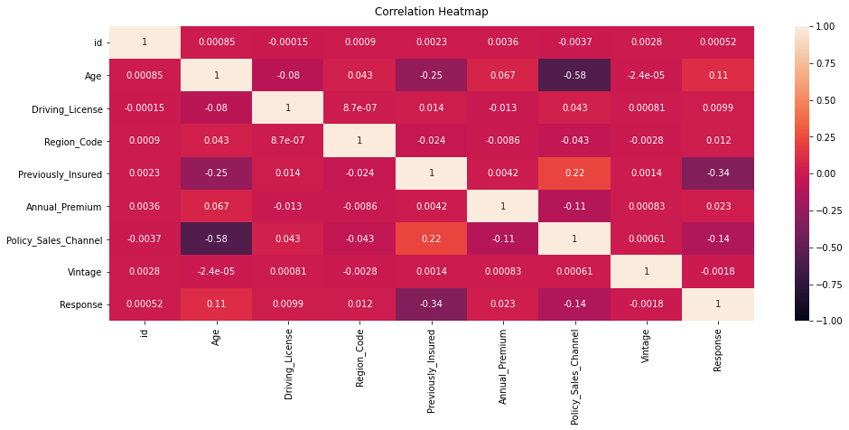
The attributes that are highly correlated with “Response” are “Previously_Insured”, Policy_Sales_Channel” and “Age”, in that order.
1
2
| #plot distribution of age as an histogram
sns.histplot(x=train["Age"], bins=20)
|
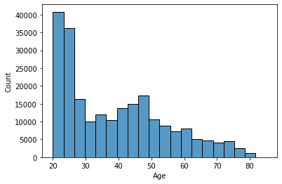
From the graph above, the histogram of age is right skewed upon inspection.
1
2
| #plot distribution of annual premium as an histogram
sns.boxplot(y=train["Age"])
|
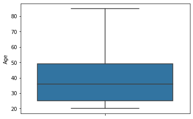
From the above boxplot, it can be seen that there are no outliers present in the Age distribution.
1
2
| #plot distribution of annual premium as an histogram
sns.histplot(x=train["Annual_Premium"], bins=20)
|
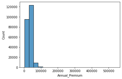
The histogram for Annual Premium also shows that it is right skewed similar to age.
1
2
| #plot distribution of annual premium as an histogram
sns.boxplot(y=train["Annual_Premium"])
|
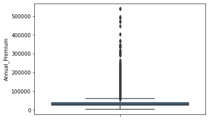
From the above boxplot on Annual premium, it can be seen that there are a large number of outliers present in the annual premium distribution.
1
2
| #plotting the distribution of gender based on customer's response
sns.catplot(x="Gender", col="Response", kind="count", data=train)
|
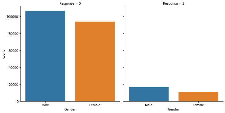
From the graph above, it can be seen that there are more number of male customers in the dataset and also male customers are more interested in vehicle insurance than female customers.
1
2
| #plotting the distribution of vehicle age based on customer's response
sns.catplot(x="Vehicle_Age", col="Response", kind="count", data=train)
|
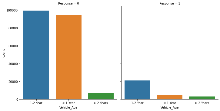
The above graph describes the distribution of Vehicle Age among the customers in the dataset. It can be seen that there are more number of customers with vehicles with 1-2 years old and less than 1 year old. The customers with vehicles greater than 2 years are significantly less. The same trend follows with the customers who responded saying that they would be interested in vehicle insurance.
1
2
| #total number of responses under each category in vehicle age
train['Vehicle_Age'].value_counts()
|
1
2
3
4
| 1-2 Year 120131
< 1 Year 98879
> 2 Years 9655
Name: Vehicle_Age, dtype: int64
|
From the above values, it can be seen that the customers with vehicles more than 2 years old are significantly less.
1
2
| #plotting the distribution of vehicle damage based on customer's response
sns.catplot(x="Vehicle_Damage", col="Response", kind="count", data=train)
|
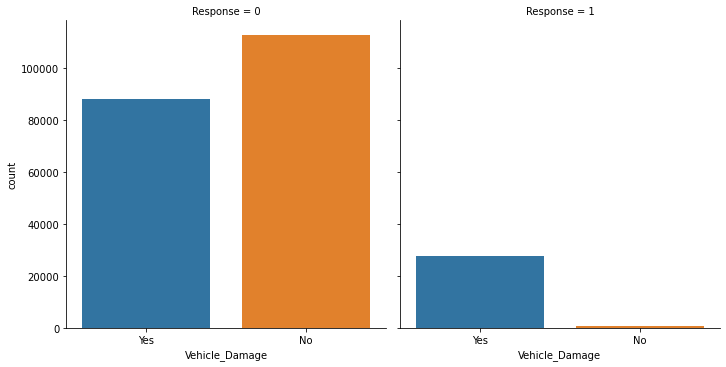
The above graph describes the number of customers that have had their vehicle damaged.
1
2
| #plotting the distribution of previosuly owned vehicle insurance based on customer's response
sns.catplot(x="Previously_Insured", col="Response", kind="count", data=train)
|
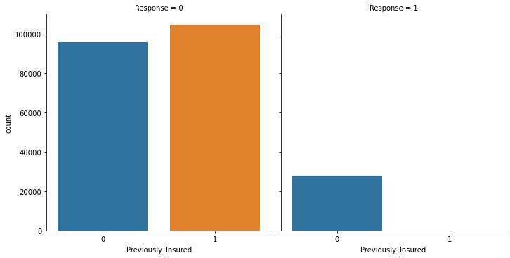
The above graph illustrates the number of customers in the dataset who already have a vehilce insurance. It can be seen that there are more customers in total who do not already have a vehicle insurance. Looking at the case of customers who are interested in a vehicle insurance, it is evident that customers who do not already own a vehicle insurance are more interested in getting a vehicle insurance.
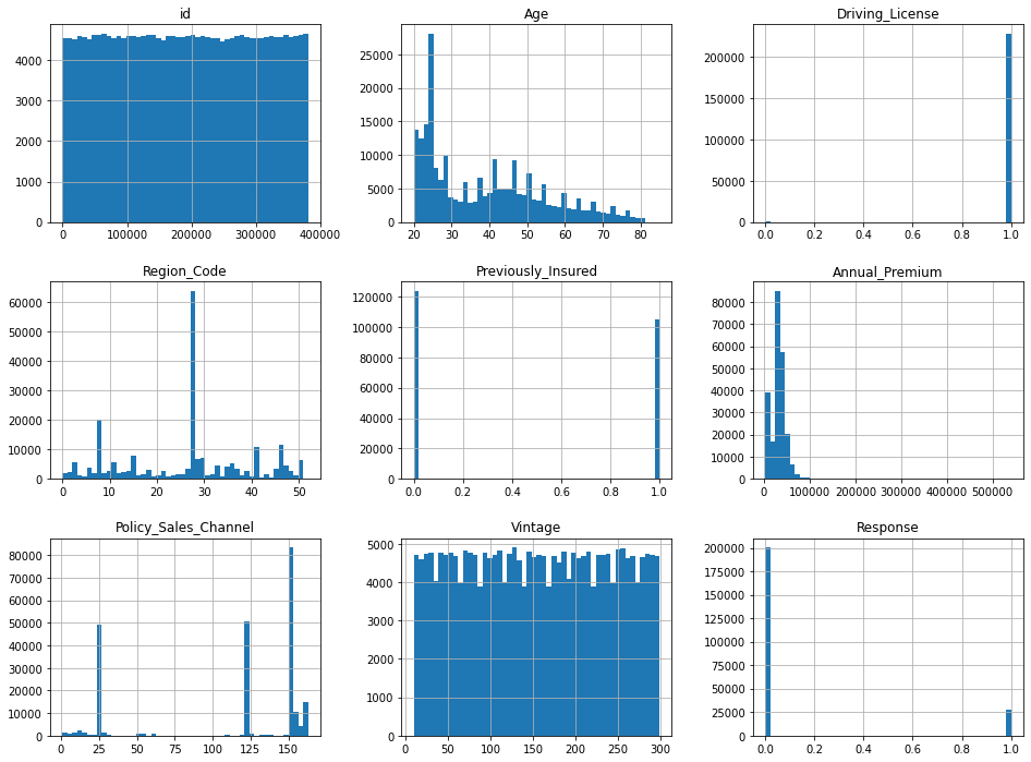
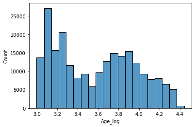
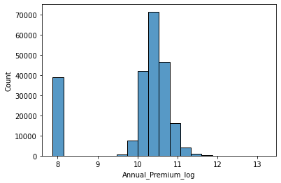
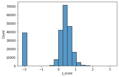
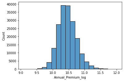
From the analysis in previous sections, there are no missing values in the dataset. Therefore, the only data preprocessing steps that needs to be taken care of is dropping the id column, data transformation of right skewed columns (Age and Annual_Premium), the removal of outliers and data scaling of the continuous variables in both train and test dataset.
1
2
| #display all numerical values in an histogram
dummy = train.hist(bins=50, figsize=(16,12))
|
1
2
| #drop the id-column in the train dataset
train = train.drop(['id'], axis = 1)
|
1
2
| #drop the id-column in the test dataset
test = test.drop(['id'], axis = 1)
|
1
2
3
4
5
6
7
8
9
10
11
12
13
14
15
16
17
| #changing categorical variables to numerical
train.loc[train['Gender'] == 'Male', 'Gender'] = 1
train.loc[train['Gender'] == 'Female', 'Gender'] = 0
test.loc[test['Gender'] == 'Male', 'Gender'] = 1
test.loc[test['Gender'] == 'Female', 'Gender'] = 0
train.loc[train['Vehicle_Age'] == '> 2 Years', 'Vehicle_Age'] = 2
train.loc[train['Vehicle_Age'] == '1-2 Year', 'Vehicle_Age'] = 1
train.loc[train['Vehicle_Age'] == '< 1 Year', 'Vehicle_Age'] = 0
test.loc[test['Vehicle_Age'] == '> 2 Years', 'Vehicle_Age'] = 2
test.loc[test['Vehicle_Age'] == '1-2 Year', 'Vehicle_Age'] = 1
test.loc[test['Vehicle_Age'] == '< 1 Year', 'Vehicle_Age'] = 0
train.loc[train['Vehicle_Damage'] == 'Yes', 'Vehicle_Damage'] = 1
train.loc[train['Vehicle_Damage'] == 'No', 'Vehicle_Damage'] = 0
test.loc[test['Vehicle_Damage'] == 'Yes', 'Vehicle_Damage'] = 1
test.loc[test['Vehicle_Damage'] == 'No', 'Vehicle_Damage'] = 0
|
1
2
3
| #changing all the dtypes to int in train dataset
for col in train.columns:
train[col] = train[col].astype(np.int32)
|
1
2
3
| #changing all the dtypes to int in test dataset
for col in test.columns:
test[col] = test[col].astype(np.int32)
|
1
2
| #log transformation of Age column
train['Age_log'] = np.log(train['Age'])
|
1
2
| #plot distribution of Age after log transformation in an histogram
sns.histplot(x=train["Age_log"], bins=20)
|
1
2
| #log transformation of Age column in the test dataset
test['Age_log'] = np.log(test['Age'])
|
1
2
| #log transformation of Annual_Premium column in train dataset
train['Annual_Premium_log'] = np.log(train['Annual_Premium'])
|
1
2
| #plot distribution of Annual_Premium after log transformation in an histogram
sns.histplot(x=train["Annual_Premium_log"], bins=20)
|
1
2
3
| #removing outliers from Annual_Premium_log using z_score
from scipy import stats
train['z_score']=stats.zscore(train['Annual_Premium_log'])
|
1
2
| #checking the distribution of z_score so that values with high z_score can be removed
sns.histplot(x=train['z_score'], bins=20)
|
1
2
| #removing values with z_score greater than 2
train = train.loc[train['z_score']<=2]
|
1
2
| #removing values with z_score lesser than -1
train = train.loc[train['z_score']>=-1]
|
1
2
| #plot distribution of Annual_Premium after removal of outliers in an histogram
sns.histplot(x=train["Annual_Premium_log"], bins=20)
|
1
2
| #log transformation of Annual_Premium column in the test dataset
test['Annual_Premium_log'] = np.log(test['Annual_Premium'])
|
1
2
3
| #drop the age column in test and train dataset
train = train.drop(['Age'], axis = 1)
test = test.drop(['Age'], axis = 1)
|
1
2
3
| #drop the Annual_Premium column from the train and test dataset
train = train.drop(['Annual_Premium'], axis = 1)
test = test.drop(['Annual_Premium'], axis = 1)
|
1
2
| #drop the z_score column from train dataset
train = train.drop(['z_score'], axis = 1)
|
1
2
3
4
5
6
7
8
9
10
11
12
13
14
15
| #data scaling needs to be done for both train and test dataset using standard scaler
from sklearn.preprocessing import StandardScaler
scaler = StandardScaler()
train_target = train['Response'].values
train_predictors = train.drop(['Response'], axis=1)
#fit_transform returns a NumPy aray, so need to put it back
#into a Pandas dataframe
scaled_vals = scaler.fit_transform(train_predictors)
train = pd.DataFrame(scaled_vals, columns=train_predictors.columns)
#put the non-scaled target back in
train['Response'] = train_target
|
1
2
3
4
5
6
7
8
| #repeat the same steps for the test dataset
test_target = test['Response'].values
test_predictors = test.drop(['Response'], axis=1)
scaled_vals = scaler.fit_transform(test_predictors)
test = pd.DataFrame(scaled_vals, columns=test_predictors.columns)
test['Response'] = test_target
|
1
2
| #plotting all the distribution of values in each column after data-preprocesing
dummy = train.hist(bins=50, figsize=(16,12))
|
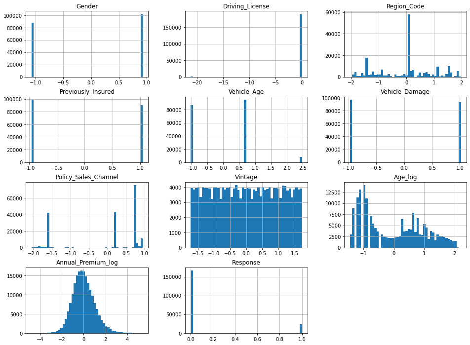
The train and test dataset is now clean and ready to be used for modeling the predictive models.
1
| train.to_csv('train.csv', index=False)
|
1
| test.to_csv('test.csv', index=False)
|
5. Modeling
The aim now is to implement and evaluate several alternative predictive models to predict whether an existing customer would be interested or not in Vehicle Insurance with the help of the predictors: Gender, Age, Driving License, Region Code, Previously Insured, Vehicle Age, Vehicle Damage, Annual Premium, Policy Sales Channel and Vintage.
1
2
3
4
5
6
|
import time #for getting local time from the number of seconds elapsed
#load the required train and test datasets
train = pd.read_csv('train.csv')
test = pd.read_csv('test.csv')
|
| Gender | Driving_License | Region_Code | Previously_Insured | Vehicle_Age | Vehicle_Damage | Policy_Sales_Channel | Vintage | Age_log | Annual_Premium_log | Response |
|---|
| 0 | 0.930654 | 0.047053 | -1.197614 | -0.956976 | 0.724263 | 1.022372 | 0.228267 | 0.210398 | 0.871617 | -0.345003 | 0 |
|---|
| 1 | -1.074513 | 0.047053 | -0.654205 | 1.044959 | -1.025121 | -0.978117 | 0.747745 | -0.852524 | -0.785843 | -0.331879 | 0 |
|---|
| 2 | 0.930654 | 0.047053 | -0.654205 | -0.956976 | 0.724263 | 1.022372 | -1.589904 | -1.461615 | 0.489337 | -0.459352 | 1 |
|---|
| 3 | 0.930654 | 0.047053 | -1.818652 | 1.044959 | -1.025121 | -0.978117 | 0.896167 | -0.780867 | -0.785843 | -1.036554 | 0 |
|---|
| 4 | -1.074513 | 0.047053 | -1.896282 | 1.044959 | -1.025121 | -0.978117 | 0.747745 | -1.354128 | -0.598007 | 1.223449 | 0 |
|---|
1
2
3
4
5
6
7
8
9
10
11
12
13
14
15
16
17
18
| <class 'pandas.core.frame.DataFrame'>
RangeIndex: 189674 entries, 0 to 189673
Data columns (total 11 columns):
# Column Non-Null Count Dtype
--- ------ -------------- -----
0 Gender 189674 non-null float64
1 Driving_License 189674 non-null float64
2 Region_Code 189674 non-null float64
3 Previously_Insured 189674 non-null float64
4 Vehicle_Age 189674 non-null float64
5 Vehicle_Damage 189674 non-null float64
6 Policy_Sales_Channel 189674 non-null float64
7 Vintage 189674 non-null float64
8 Age_log 189674 non-null float64
9 Annual_Premium_log 189674 non-null float64
10 Response 189674 non-null int64
dtypes: float64(10), int64(1)
memory usage: 15.9 MB
|
Sampling
The train and test dataset are too large and would take massive amounts of time to train models on this dataset. Therefore, a sample is taken out of the train and test dataset.
1
2
| #sampling from train dataset
ftrain = train.sample(n=50000, random_state=7)
|
| Gender | Driving_License | Region_Code | Previously_Insured | Vehicle_Age | Vehicle_Damage | Policy_Sales_Channel | Vintage | Age_log | Annual_Premium_log | Response |
|---|
| 50183 | 0.930654 | 0.047053 | -1.430503 | 1.044959 | -1.025121 | -0.978117 | 0.729192 | 1.416637 | -1.096595 | 0.815633 | 0 |
|---|
| 46028 | 0.930654 | 0.047053 | -1.430503 | 1.044959 | -1.025121 | -0.978117 | 0.747745 | -0.374806 | -0.988722 | 2.021025 | 0 |
|---|
| 41101 | -1.074513 | 0.047053 | 0.587873 | -0.956976 | -1.025121 | -0.978117 | 0.747745 | 0.735888 | -0.509064 | -0.685612 | 0 |
|---|
| 39742 | -1.074513 | 0.047053 | 0.122094 | -0.956976 | 0.724263 | 1.022372 | -1.589904 | 0.819489 | 0.547607 | 2.429836 | 1 |
|---|
| 187634 | 0.930654 | 0.047053 | -0.343685 | 1.044959 | -1.025121 | -0.978117 | 0.896167 | 0.640345 | -1.327174 | 0.145065 | 0 |
|---|
1
2
| #sampling from test dataset
ftest = test.sample(n=35000, random_state=7)
|
| Gender | Driving_License | Region_Code | Previously_Insured | Vehicle_Age | Vehicle_Damage | Policy_Sales_Channel | Vintage | Age_log | Annual_Premium_log | Response |
|---|
| 140791 | 0.922772 | 0.045936 | 0.122655 | -0.919475 | -1.074838 | 0.991209 | 0.220503 | -0.864108 | -1.257842 | -0.084741 | 1 |
|---|
| 21139 | -1.083691 | 0.045936 | -1.161235 | -0.919475 | 0.689124 | 0.991209 | -1.587009 | 1.170042 | 0.518490 | 1.032980 | 1 |
|---|
| 12854 | -1.083691 | 0.045936 | -0.028391 | 1.087577 | -1.074838 | -1.008869 | 0.884487 | -0.253863 | -0.829732 | -2.127575 | 0 |
|---|
| 13704 | 0.922772 | 0.045936 | 1.482068 | 1.087577 | -1.074838 | -1.008869 | 0.884487 | -0.026517 | -1.377059 | -0.049361 | 0 |
|---|
| 21554 | 0.922772 | 0.045936 | -0.406006 | -0.919475 | 0.689124 | 0.991209 | -1.587009 | -1.306835 | 0.896837 | 0.597470 | 0 |
|---|
Train Models
The first step is to create seperate arrays for the predictors (Xtrain) and for the target (ytrain):
1
2
3
4
5
6
| from sklearn.model_selection import GridSearchCV
#seperating the predictors and target variable
Xtrain = ftrain.drop('Response', axis=1)
ytrain = ftrain['Response'].copy()
|
Baseline Model
A majority class classifier is used as baseline where most common class label in the training set would be found out and predicted as the output always.
1
2
| #count the number of instances
ftrain["Response"].value_counts()
|
1
2
3
| 0 43867
1 6133
Name: Response, dtype: int64
|
0: Not interested, 1: Interested
1
2
| #train set size
ftrain.shape[0]
|
According to the baseline classifier, the output will be “Not interested” for all predictions. In this project, macro-averaging will be used (precision, recall and F-score are evaluated in each class seperately and then avergaed across classes).
Therefore, applying the baseline classifier to all of the train dataset.
For responses with “Not interested”, the accuarcy measures will be:
- Precision: 43867/50000 = 0.877
- Recall: 50000/50000 = 1.0
- F-score: 2/(1/precision+1/recall) = 0.935
For responses with “Interested”, the accuarcy measures will be:
- Precision: 0.0/0.0 = 0.0
- Recall: 0.0/6133 = 0.0
- F-score: 0.0
The averages of the two classes which is the eventual baseline scores, are:
- Precision: 0.439
- Recall: 0.5
- F-score: 0.468
Random Forest
1
2
3
4
5
6
7
8
9
10
11
12
13
14
15
16
17
18
19
20
21
| from sklearn.ensemble import RandomForestClassifier
rf = RandomForestClassifier()
#put in the hyperparameters
param_grid = {
'n_estimators': [10, 100, 200, 1000],
'max_depth': [3, 5, 15],
'min_samples_split': [5, 10],
'random_state': [7]
}
#5-fold cross-validation is used
grid_search = GridSearchCV(rf, param_grid, cv=5,
scoring='f1_macro',
return_train_score=True)
start = time.time()
grid_search.fit(Xtrain, ytrain)
end = time.time() - start
print(f"Took {end} seconds")
|
1
| Took 899.0751824378967 seconds
|
1
| grid_search.best_estimator_
|
1
2
| RandomForestClassifier(max_depth=15, min_samples_split=5, n_estimators=10,
random_state=7)
|
1
| grid_search.best_score_
|
The best hyperparameters prove to be n_estimators = 200, max_depth = 15 and min_sample_split=5. Based on this, they achieve a F-score of 0.51 which is the best one so far.
The results of the best model are recorded in each split and the below command gives the index of the best performing model,
1
| grid_search.cv_results_['rank_test_score'].tolist().index(1)
|
1
2
3
4
5
| rf_split_test_scores = []
for x in range(5):
#extract f-score of the best model (index=18) from each of the 5 splits
val = grid_search.cv_results_[f"split{x}_test_score"][18]
rf_split_test_scores.append(val)
|
The scores achieved by all the models for different hyperparameter are reviewed:
1
2
3
4
5
6
| val_scores = grid_search.cv_results_['mean_test_score']
train_scores = grid_search.cv_results_['mean_train_score']
params = [str(x) for x in grid_search.cv_results_["params"]]
for val_score, train_score, param in sorted(zip(val_scores, train_scores, params), reverse=True):
print(val_score, train_score, param)
|
1
2
3
4
5
6
7
8
9
10
11
12
13
14
15
16
17
18
19
20
21
22
23
24
| 0.5077910772485159 0.6144937097675991 {'max_depth': 15, 'min_samples_split': 5, 'n_estimators': 10, 'random_state': 7}
0.500160391905794 0.5800966185190405 {'max_depth': 15, 'min_samples_split': 10, 'n_estimators': 10, 'random_state': 7}
0.4901043794684668 0.5983222542940497 {'max_depth': 15, 'min_samples_split': 5, 'n_estimators': 100, 'random_state': 7}
0.489769462731983 0.5974611399846733 {'max_depth': 15, 'min_samples_split': 5, 'n_estimators': 200, 'random_state': 7}
0.488091595400079 0.5962736744561885 {'max_depth': 15, 'min_samples_split': 5, 'n_estimators': 1000, 'random_state': 7}
0.48802775984303126 0.565265257292125 {'max_depth': 15, 'min_samples_split': 10, 'n_estimators': 200, 'random_state': 7}
0.4879105683806045 0.5624624248068428 {'max_depth': 15, 'min_samples_split': 10, 'n_estimators': 1000, 'random_state': 7}
0.487125083987973 0.5651251866402451 {'max_depth': 15, 'min_samples_split': 10, 'n_estimators': 100, 'random_state': 7}
0.4673314366705239 0.46733143701057855 {'max_depth': 5, 'min_samples_split': 5, 'n_estimators': 200, 'random_state': 7}
0.4673314366705239 0.46733143701057855 {'max_depth': 5, 'min_samples_split': 5, 'n_estimators': 1000, 'random_state': 7}
0.4673314366705239 0.46733143701057855 {'max_depth': 5, 'min_samples_split': 5, 'n_estimators': 100, 'random_state': 7}
0.4673314366705239 0.46733143701057855 {'max_depth': 5, 'min_samples_split': 5, 'n_estimators': 10, 'random_state': 7}
0.4673314366705239 0.46733143701057855 {'max_depth': 5, 'min_samples_split': 10, 'n_estimators': 200, 'random_state': 7}
0.4673314366705239 0.46733143701057855 {'max_depth': 5, 'min_samples_split': 10, 'n_estimators': 1000, 'random_state': 7}
0.4673314366705239 0.46733143701057855 {'max_depth': 5, 'min_samples_split': 10, 'n_estimators': 100, 'random_state': 7}
0.4673314366705239 0.46733143701057855 {'max_depth': 5, 'min_samples_split': 10, 'n_estimators': 10, 'random_state': 7}
0.4673314366705239 0.46733143701057855 {'max_depth': 3, 'min_samples_split': 5, 'n_estimators': 200, 'random_state': 7}
0.4673314366705239 0.46733143701057855 {'max_depth': 3, 'min_samples_split': 5, 'n_estimators': 1000, 'random_state': 7}
0.4673314366705239 0.46733143701057855 {'max_depth': 3, 'min_samples_split': 5, 'n_estimators': 100, 'random_state': 7}
0.4673314366705239 0.46733143701057855 {'max_depth': 3, 'min_samples_split': 5, 'n_estimators': 10, 'random_state': 7}
0.4673314366705239 0.46733143701057855 {'max_depth': 3, 'min_samples_split': 10, 'n_estimators': 200, 'random_state': 7}
0.4673314366705239 0.46733143701057855 {'max_depth': 3, 'min_samples_split': 10, 'n_estimators': 1000, 'random_state': 7}
0.4673314366705239 0.46733143701057855 {'max_depth': 3, 'min_samples_split': 10, 'n_estimators': 100, 'random_state': 7}
0.4673314366705239 0.46733143701057855 {'max_depth': 3, 'min_samples_split': 10, 'n_estimators': 10, 'random_state': 7}
|
The performance of Random Forest varies between 0.47 and 0.51. It can also be noticed that better score is achieved for greater max_depth. However, this score is only slight better than the baseline model. Therefore, more models need to evaluted for better understanding.
1
2
3
4
5
6
7
8
| # put them into a separate variable for convenience
feature_importances = grid_search.best_estimator_.feature_importances_
# the order of the features in `feature_importances` is the same as in the Xtrain dataframe,
# so we can "zip" the two and print in the descending order:
for k, v in sorted(zip(feature_importances, Xtrain.columns), reverse=True):
print(f"{v}: {k}")
|
1
2
3
4
5
6
7
8
9
10
| Vehicle_Damage: 0.23034578200483757
Age_log: 0.15910325280867196
Annual_Premium_log: 0.1399068056819435
Previously_Insured: 0.13163255776225508
Vintage: 0.11583783732321544
Policy_Sales_Channel: 0.08475334501851194
Region_Code: 0.06984894911839537
Vehicle_Age: 0.05473726453721193
Gender: 0.012907136629646949
Driving_License: 0.0009270691153103203
|
Vehicle damage, age, annual premium, previously insured and vintage are quite predictive of whether a customer would be interested in vehicle insurance or not.
Every other variable has very little to do with the response of the customer.
Following on, the model is saved to the disk so that it can be used in the future directly for testing instead of re-training the model.
1
2
3
4
5
6
7
8
| import os
from joblib import dump
#creating a folder to save all the models
if not os.path.exists('ML models'):
os.makedirs('ML models')
dump(grid_search.best_estimator_, 'ML models/rf-clf.joblib')
|
1
| ['ML models/rf-clf.joblib']
|
The model will be loaded later on using joblib’s load function.
Support Vector Machines
Linear SVMs
1
2
3
4
5
6
7
8
9
10
11
12
13
14
15
16
17
18
19
20
| from sklearn.svm import LinearSVC
lsvm = LinearSVC()
# specify the hypermaters
param_grid = {
'C': [0.1, 1, 3, 5],
'max_iter': [5000],
'random_state': [7]
}
#5-fold cross-validation is used
grid_search = GridSearchCV(lsvm, param_grid, cv=5,
scoring='f1_macro',
return_train_score=True)
start = time.time()
grid_search.fit(Xtrain, ytrain)
end = time.time() - start
print(f"Took {end} seconds")
|
1
| Took 498.01508927345276 seconds
|
1
| grid_search.best_estimator_
|
1
| LinearSVC(C=0.1, max_iter=5000, random_state=7)
|
1
| grid_search.best_score_
|
There is no significant difference between the f-score of the Linear SVM and the baseline model. Therefore, this model turns out to be very poor.
1
2
3
4
5
6
| val_scores = grid_search.cv_results_["mean_test_score"]
train_scores = grid_search.cv_results_["mean_train_score"]
params = [str(x) for x in grid_search.cv_results_["params"]]
for val_score, train_score, param in sorted(zip(val_scores, train_scores, params), reverse=True):
print(val_score, train_score, param)
|
1
2
3
4
| 0.4673314366705239 0.46733143701057855 {'C': 3, 'max_iter': 5000, 'random_state': 7}
0.4673314366705239 0.46733143701057855 {'C': 1, 'max_iter': 5000, 'random_state': 7}
0.4673314366705239 0.46733143701057855 {'C': 0.1, 'max_iter': 5000, 'random_state': 7}
0.46732576201501475 0.4673662960221964 {'C': 5, 'max_iter': 5000, 'random_state': 7}
|
From the above results, it can be seen that there is no difference in the F-score as the C-value changes.
However, this model is now saved for future refernece.
1
2
3
4
5
6
7
8
| import os
from joblib import dump
# create a folder where all trained models will be kept
if not os.path.exists("ML models"):
os.makedirs("ML models")
dump(grid_search.best_estimator_, 'ML models/svm-lnr-clf.joblib')
|
1
| ['ML models/svm-lnr-clf.joblib']
|
Radial Basis Function
1
2
3
4
5
6
7
8
9
10
11
12
13
14
15
16
17
18
19
20
21
| from sklearn.svm import SVC
svm = SVC()
#put in the parameters
param_grid = {
'C': [1, 10, 100],
'gamma': ["scale", "auto"],
'kernel': ["rbf"],
'random_state': [7]
}
#5-fold cross-validation is used
grid_search = GridSearchCV(svm, param_grid, cv=5,
scoring='f1_macro',
return_train_score=True)
start = time.time()
grid_search.fit(Xtrain, ytrain)
end = time.time() - start
print(f"Took {end} seconds")
|
1
| Took 5844.312863826752 seconds
|
This model took significant amount of time to train and are impartical for large datasets.
1
| grid_search.best_estimator_
|
1
| SVC(C=100, gamma='auto', random_state=7)
|
1
| grid_search.best_score_
|
The F-score of this model is approximately 0.475 which is 0.01 more than that of the baseline model. Therefore, this model turns out to be no better than the baseline model as well.
1
2
3
4
5
6
7
| # obtain the f-scores of the best models in each split
svmrbf_split_test_scores = []
for x in range(5):
# extract f-score of the best model (at index=0) from each of the 5 splits
val = grid_search.cv_results_[f"split{x}_test_score"][0]
svmrbf_split_test_scores.append(val)
|
1
2
3
4
5
6
| val_scores = grid_search.cv_results_["mean_test_score"]
train_scores = grid_search.cv_results_["mean_train_score"]
params = [str(x) for x in grid_search.cv_results_["params"]]
for val_score, train_score, param in sorted(zip(val_scores, train_scores, params), reverse=True):
print(val_score, train_score, param)
|
1
2
3
4
5
6
| 0.4752675855876845 0.49304582093749144 {'C': 100, 'gamma': 'auto', 'kernel': 'rbf', 'random_state': 7}
0.4749530799050228 0.49179605580100966 {'C': 100, 'gamma': 'scale', 'kernel': 'rbf', 'random_state': 7}
0.4682958744065912 0.47032797495572937 {'C': 10, 'gamma': 'auto', 'kernel': 'rbf', 'random_state': 7}
0.4682958744065912 0.470081072861702 {'C': 10, 'gamma': 'scale', 'kernel': 'rbf', 'random_state': 7}
0.4673314366705239 0.46733143701057855 {'C': 1, 'gamma': 'scale', 'kernel': 'rbf', 'random_state': 7}
0.4673314366705239 0.46733143701057855 {'C': 1, 'gamma': 'auto', 'kernel': 'rbf', 'random_state': 7}
|
From the above results, it can be seen that the F-scores of the model increase with increase in the C - value. This is similar to that of random forests where high values of dept produced better results.
Polynomial SVM was ignored as it took a significant amount of time to train.
The SVM rbf model is saved.
1
2
3
4
5
6
7
8
| import os
from joblib import dump
# create a folder where all trained models will be kept
if not os.path.exists("ML models"):
os.makedirs("ML models")
dump(grid_search.best_estimator_, 'ML models/svm-rbf-clf.joblib')
|
1
| ['ML models/svm-rbf-clf.joblib']
|
From the two SVM models above, the F-scores are less than what was observed for Random forest and are not significantly different from the baseline models. Compared to the SVM models, the random forest was slightly better with an F-score of 0.51. However, this is an extremly poor score as well in reality. A model with such poor score has significantly low prediction power.
Test the Models
Even though, models that were trained have a poor f-score, the random forest with the relatively high f-score will be evaluated on the test dataset.
The model is loaded from the local disk:
1
2
3
| from joblib import load
best_rf = load("ML models/rf-clf.joblib")
|
1
2
3
| # drop labels for training set, but keep all others
Xtest = ftest.drop("Response", axis=1)
ytest = ftest["Response"].copy()
|
1
2
3
4
5
6
7
8
9
10
11
| from sklearn.metrics import precision_recall_fscore_support
# rf
yhat = best_rf.predict(Xtest)
# micro-averaged precision, recall and f-score
p, r, f, s = precision_recall_fscore_support(ytest, yhat, average="macro")
print("Random Forest:")
print(f"Precision: {p}")
print(f"Recall: {r}")
print(f"F score: {f}")
|
1
2
3
4
| Random Forest:
Precision: 0.6461335174851621
Recall: 0.5258023688231142
F score: 0.5218418455618304
|
Thus, similar classification accuracy can be found with Random forrest classifier, as observed during cross-validation.
6. Future Improvements and Business Scenario
There is big room for future improvments for the model as the models accuracy is very poor. Different steps need to be taken to overcome this problem. One of the reason for this poor score could be that fact that there was significantly low number of customers interested in vehicle insurance compared to customers who weren’t. This could have potentially created a bias in the models learning. Another problem is that the predictors may not be a good representative of the target variable. To support this, the correlation matrix in the group report showed very poor correlation between the target variable and the predictors. Addressing these problesm could be potential future improvements.
Currently, this model cannot be used in real world scenarios due to its low accuarcy but similar models with high accuracy can be used in various business scenarios. For example, banks can use this type of model to predict who would be interested in a certain type of credit or debit cards.
